The crosswise model
Crosswise questions let respondents answer a sensitive question
without revealing their answer directly. A respondent is shown a
sensitive statement and a second statement whose prevalence is known
(p). They report only whether their answers to the two
statements are the same or different. The crosswise response is
therefore not itself the sensitive-trait indicator.
The design protects privacy, but it also makes inattentive responses
important: respondents who answer at random pull the observed crosswise
proportion toward one half. cWise uses an anchor
crosswise question with known sensitive-item prevalence to estimate
attentiveness and correct that bias.
The package includes simulated data from this design. Y
is the primary crosswise response, A is the anchor
response, and p and p.prime are the known
randomization probabilities.
head(cmdata)
#>   Y A weight    p p.prime
#> 1 1 1   1.25 0.15    0.15
#> 2 0 0   1.25 0.15    0.15
#> 3 0 0   1.25 0.15    0.15
#> 4 1 0   5.00 0.15    0.15
#> 5 0 1   1.25 0.15    0.15
#> 6 1 1   1.25 0.15    0.15
Estimate prevalence
Use bc_est() to obtain both the naive and bias-corrected
prevalence estimates. Here, the anchor makes it possible to estimate the
share of attentive respondents as well.
estimate <- bc_est(Y = Y, A = A, p = 0.15, p.prime = 0.15, data = cmdata)
estimate
#> $Results
#>                 Estimate Std. Error 95%CI(Low) 95%CI(Up)
#> Naive Crosswise   0.1950     0.0144     0.1667    0.2233
#> Bias-Corrected    0.1054     0.0214     0.0679    0.1529
#>
#> $Stats
#>  Attentive Rate Sample Size
#>          0.7729        2000
Results contains point estimates, standard errors, and
confidence intervals. Stats reports the estimated
attentive-response rate and the analysis sample size. The bias-corrected
row is usually the estimand of interest when the anchor-question
assumptions are credible.
Sensitivity analysis without an anchor
When no anchor question was fielded, cmBound() shows how
the estimate changes over a plausible range of inattentive-response
rates. The following calculation uses only the observed primary-question
proportion, its randomization probability, and the sample size.
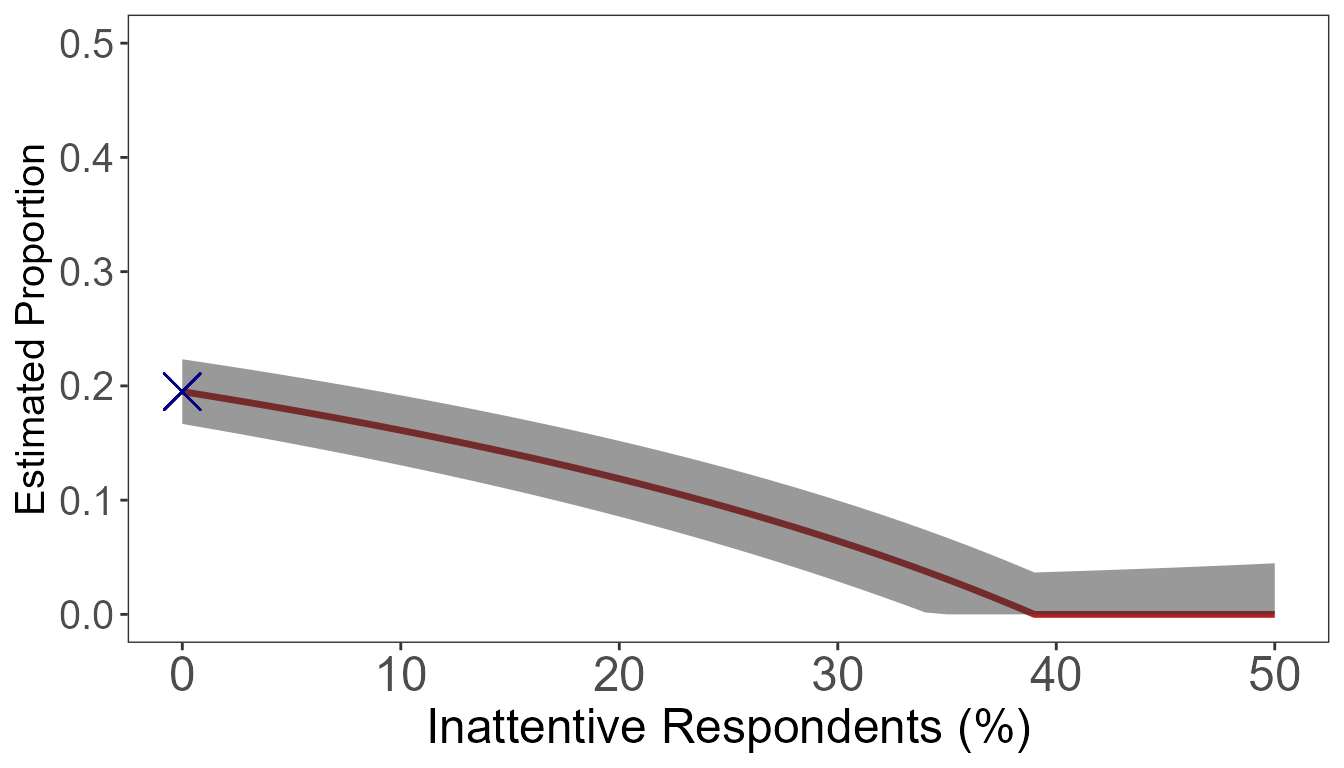
An optional direct-question estimate can be supplied with
dq and N.dq; it is then drawn as a reference
line with its uncertainty interval.
Simulation and power planning
Power-analysis functions are deliberately not evaluated while this
vignette is built: they run nested bootstrap simulations. Start with a
small exploratory run and increase N.sim for a
study-planning analysis.
simulation <- sim_cwdata(
  N.sim = 200, sample = 500, prevalence = 0.10, p = 0.15, p.prime = 0.15,
  gamma = 0.80, direct = 0.05
)
simulation$Results

sim_power(
  N.sim = 500, sample = 1000, pi.null = 0.05, pi.alt = 0.10,
  p = 0.15, p.prime = 0.15, gamma = 0.80, direct = 0.05
)
sim_estimates() plots the simulated estimates, while
sim_power_N() compares the package’s standard sample-size
grid. These functions are intended for interactive study planning rather
than a package build.
The sensitive trait in a crosswise survey is latent: we observe
crosswise and anchor responses, not each respondent’s trait status.
cmreg() and cmreg_p() fit likelihood-based
models that account for this measurement structure.
The latent trait as an outcome
cmreg() models the probability of possessing the
sensitive trait as a function of covariates. The formula contains the
primary crosswise response on the left; supply the anchor response
separately.
outcome_fit <- cmreg(
  Y ~ female + age,
  anchor = A, p = 0.10, p.prime = 0.15,
  data = cmdata2, n.start = 1L
)
summary(outcome_fit)
#> Coefficients:
#>             Estimate Std. Error z score Pr(>|z|)
#> (Intercept)  -1.6501     0.4266 -3.8684   0.0001
#> female        0.2813     0.1427  1.9717   0.0486
#> age           0.0326     0.0133  2.4505   0.0143
#>
#> Auxiliary coefficients:
#>             Estimate Std. Error z score Pr(>|z|)
#> (Intercept)   0.1405     1.1363  0.1237   0.9016
#> female       -0.2059     0.4121 -0.4995   0.6174
#> age           0.0594     0.0394  1.5074   0.1317
The first coefficient block describes the latent trait. The auxiliary block describes the probability of attentive responding. Predict trait prevalence at specific covariate combinations with uncertainty from a parametric bootstrap.
trait_predictions <- cmpredict(
  outcome_fit,
  newdata = data.frame(female = c(0, 1), age = c(30, 30)),
  nsim = 300, seed = 20260825
)
trait_predictions
#>    estimate  conf.low conf.high
#> 1 0.3381928 0.3046601 0.3790037
#> 2 0.4037005 0.3565547 0.4515935
The plot shows the estimated prevalence and its 95% parametric-bootstrap interval for each covariate scenario.
trait_labels <- c("Female = 0", "Female = 1")
plot(
  seq_len(nrow(trait_predictions)), trait_predictions$estimate,
  ylim = c(0, 1), xlim = c(0.75, 2.25), xaxt = "n",
  xlab = "Covariate scenario", ylab = "Predicted trait prevalence",
  pch = 19, col = "#1B6CA8"
)
axis(1, at = seq_along(trait_labels), labels = trait_labels)
arrows(
  x0 = seq_len(nrow(trait_predictions)), y0 = trait_predictions$conf.low,
  x1 = seq_len(nrow(trait_predictions)), y1 = trait_predictions$conf.high,
  angle = 90, code = 3, length = 0.05, col = "#1B6CA8"
)
The latent trait as a predictor
cmreg_p() models a continuous observed outcome while
treating the sensitive trait as a latent predictor. The formula now
contains the observed outcome; the crosswise and anchor responses are
supplied by name.
predictor_fit <- cmreg_p(
  V ~ age + female,
  crosswise = Y, anchor = A, p = 0.10, p.prime = 0.15,
  data = cmdata3, n.start = 1L
)
summary(predictor_fit)
#> Coefficients:
#>             Estimate Std. Error Z score Pr(>|z|)
#> (Intercept)   0.0236     0.1478  0.1595   0.8733
#> age           0.0096     0.0048  2.0054   0.0449
#> female        0.2473     0.0520  4.7517   0.0000
#> Y             0.9859     0.0756 13.0368   0.0000
#>
#> Auxiliary coefficients:
#>             Estimate Std. Error Z score Pr(>|z|)
#> (Intercept)  -1.7342     0.4010 -4.3253   0.0000
#> age           0.0352     0.0126  2.7948   0.0052
#> female        0.2880     0.1356  2.1235   0.0337
#>
#> Additional auxiliary coefficients:
#>             Estimate Std. Error Z score Pr(>|z|)
#> (Intercept)   0.2468     1.0680  0.2311   0.8172
#> age           0.0548     0.0370  1.4821   0.1383
#> female       -0.1076     0.3779 -0.2849   0.7758
#> sigma         1.0438     0.0206 50.7779   0.0000
Predictions are returned for both latent-trait states. Each supplied covariate scenario therefore produces an “absent” and a “present” row.
outcome_predictions <- cmpredict_p(
  predictor_fit,
  newdata = data.frame(age = 30, female = 1),
  nsim = 300, seed = 20260825
)
outcome_predictions
#>                   estimate  conf.low conf.high
#> 1: trait absent  0.5600254 0.4581331 0.6481188
#> 1: trait present 1.5459544 1.4128550 1.6627413
This plot compares the model-implied observed outcome when the latent trait is absent versus present, with 95% parametric-bootstrap intervals.
state_labels <- sub("^[0-9]+: ", "", rownames(outcome_predictions))
ylim <- range(outcome_predictions$conf.low, outcome_predictions$conf.high)
plot(
  seq_len(nrow(outcome_predictions)), outcome_predictions$estimate,
  ylim = ylim + c(-0.05, 0.05), xlim = c(0.75, 2.25), xaxt = "n",
  xlab = "Latent-trait scenario", ylab = "Predicted observed outcome",
  pch = 19, col = "#A23A2E"
)
axis(1, at = seq_along(state_labels), labels = state_labels)
arrows(
  x0 = seq_len(nrow(outcome_predictions)), y0 = outcome_predictions$conf.low,
  x1 = seq_len(nrow(outcome_predictions)), y1 = outcome_predictions$conf.high,
  angle = 90, code = 3, length = 0.05, col = "#A23A2E"
)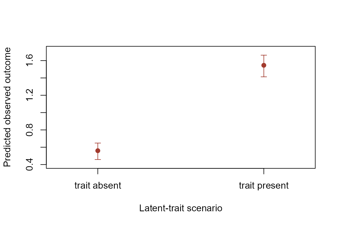
The uncertainty intervals reflect sampling uncertainty in the fitted parameters. They do not turn an individual respondent’s latent trait into an observed value; instead, they compare model-implied outcomes under the two trait scenarios.